Facial Landmark Detection in OpenCV4
Learn about the face landmark detection in OpenCV4 in this article by Roy Shilkrot, an assistant professor of computer science at Stony Brook University, where he leads the Human Interaction group. Dr. Shilkrot’s research is in computer vision, human-computer interfaces, and the cross-over between these two domains, funded by US federal, New York State, and industry grants.
Face Landmark and Pose with the Face Module
Face landmark detection is the process of finding points of interest in an image of a human face. It has recently seen rapid growth in the computer vision community because it has many compelling applications. For example, we have shown the ability to detect emotion through facial gestures, estimating gaze direction, changing facial appearance (face swap), augmenting faces with graphics, and puppeteering of virtual characters.
We can see many of these applications in today’s smartphones and PC web-camera programs. To achieve this, the landmark detector must find dozens of points on the face, such as corners of the mouth, corners of eyes, the silhouette of the jaws, and many more. Many algorithms were developed and implemented in OpenCV. In this article, we will discuss the process of face landmark (also known as facemark) detection using the cv::face module, which provides an API for inference, as well as training of a facemark detector. We will see how to apply the facemark detector to locating the direction of the face in 3D.
The code files for this article can be downloaded from https://github.com/PacktPublishing/Mastering-OpenCV-4-Third-Edition. You will need the following technologies and installations to build the code:
- OpenCV v4 (compiled with the
face contribmodule) - Boost v1.66+
To run the facemark detector, a pre-trained model is required. Although training the detector model is certainly possible with the APIs provided in OpenCV, some pre-trained models are offered for download. One such model can be obtained from https://raw.githubusercontent.com/kurnianggoro/GSOC2017/master/data/lbfmodel.yaml, supplied by the contributor of the algorithm implementation to OpenCV.
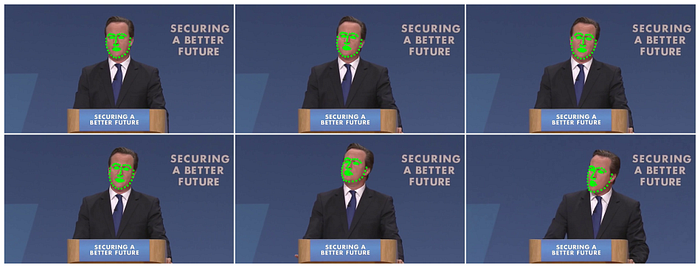
The facemark detector can work with any image. However, we can use a prescribed dataset of facial photos and videos that are used to benchmark facemark algorithms. Such a dataset is 300-VW, available through Intelligent Behaviour Understanding Group (iBUG), a computer vision group at Imperial College London: https://ibug.doc.ic.ac.uk/resources/300-VW/. It contains hundreds of videos of facial appearances in media, carefully annotated with 68 facial landmark points. This dataset can be used for training the facemark detector, as well as to understand the performance level of the pre-trained model we use. The following is an excerpt from one of the 300-VW videos with ground truth annotation:

Facial landmark detection in OpenCV
Landmark detection starts with face detection, finding faces in the image and their extents (bounding boxes). Facial detection has long been considered a solved problem, and OpenCV contains one of the first robust face detectors freely available to the public. In fact, OpenCV, in its early days, was primarily known and used for its fast face detection feature, implementing the canonical Viola-Jones boosted cascade classifier algorithm (Viola et al. 2001, 2004), and providing a pre-trained model. While face detection has grown much since those early days, the fastest and easiest method for detecting faces in OpenCV is still to use the bundled cascade classifiers by means of the cv::CascadeClassifier class provided in the core module.
We implement a simple helper function to detect faces with the cascade classifier, shown as follows:
We may want to tweak the two parameters that govern the face detection: pyramid scale factor and number of neighbors. The pyramid scale factor is used to create a pyramid of images within which the detector will try to find faces. This is how multi-scale detection is achieved since the bare detector has a fixed aperture.
In each step of the image pyramid, the image is downscaled by this factor, so a small factor (closer to 1.0) will result in many images, longer runtime, but more accurate results. We also have control of the lower threshold for a number of neighbors. This comes into play when the cascade classifier has multiple positive face classifications in close proximity.
Here, we instruct the overall classification to only return a face bound if it has at least three neighboring positive face classifications. A lower number (an integer, close to 1) will return more detections, but will also introduce false positives.
We must initialize the cascade classifier from the OpenCV-provided models (XML files of the serialized models are provided in the $OPENCV_ROOT/data/haarcascades directory). We use the standard trained classifier on frontal faces, demonstrated as follows:
A visualization of the results of the face detector is shown in the following screenshot:

The facemark detector will work around the detected faces, beginning at the bounding boxes. However, we must first initialize the cv::face::Facemark object, demonstrated as follows:
The cv::face::Facemark abstract API is used for all the landmark detector flavors and offers base functionality for implementation for inference and training according to the specific algorithm. Once loaded, the facemark object can be used with its fit function to find the face shape, shown as follows:
A visualization of the results of the landmark detector (using cv::face::drawFacemarks) is shown in the following screenshot:

Measuring error
Visually, the results seem very good. However, since we have the ground truth data, we may elect to analytically compare it to the detection and get an error estimate. We can use a standard mean Euclidean distance metric ( ) to tell how close each predicted landmark is to the ground truth on average:
float MeanEuclideanDistance(const vector<Point2f>& A, const vector<Point2f>& B) {float med = 0.0f;for (int i = 0; i < A.size(); ++i) { med += cv::norm(A[i] - B[i]);}return med / (float)A.size();}
A visualization of the results with the prediction (red) and ground truth (green) overlaid, shown in the following screenshot:

We can see the average error over all landmarks is roughly only one pixel for these particular video frames.
Estimating face direction from landmarks
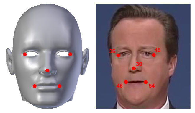
Having obtained the facial landmarks, we can attempt to find the direction of the face. The 2D face landmark points essentially conform to the shape of the head. So, given a 3D model of a generic human head, we can find approximate corresponding 3D points for a number of facial landmarks, as shown in the following photo:

Estimated pose calculation
From these 2D–3D correspondences, we can calculate 3D pose (rotation and translation) of the head, with respect to the camera, by way of the Point-n-Perspective (PnP) algorithm. The camera that took the preceding picture has a rigid transformation, meaning it has moved a certain distance from the object, as well as rotated somewhat, with respect to it. In very broad terms, we can then write the relationship between points on the image (near the camera) and the object as follows:

This is an equation where

are the object’s 3D position, and

are points in the image. This equation also includes a projection, governed by the camera intrinsic parameters (focal length f and center point c), that transforms the 3D points to 2D image points, up to scale s. Say we are given the intrinsic parameters by calibrating the camera, or we approximate them, we are left to find 12 coefficients for the rotation and translation.
If we had enough 2D and 3D corresponding points, we can write a system of linear equations, where each point can contribute two equations, to solve for all of these coefficients. In fact, it was shown that we don’t need six points, since the rotation has less than nine degrees of freedom, we can make do with just four points. OpenCV provides an implementation to find the rotation and translation with its cv::solvePnP functions of the calib3d module.
We line up the 3D and 2D points and employ cv::solvePnP:
The K matrix for the camera intrinsics we estimate from size the preceding image.
Projecting the pose on the image
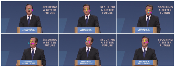
After obtaining the rotation and translation, we project four points from the object coordinate space to the preceding image: tip of the nose, x axis direction, y axis direction, and z axis direction, and draw the arrows in the preceding image:
This result in a visualization of the direction the face is pointing:

If you found this article interesting, you can explore Mastering OpenCV 4 to work on practical computer vision projects covering advanced object detector techniques and modern deep learning and machine learning algorithms. Mastering OpenCV 4, now in its third edition, targets computer vision engineers taking their first steps toward mastering OpenCV.


