Visualizing Pathfinding Algorithms with ReactJS — RapidKL MRT🚄

Transportation networks, like MRT systems, are the veins of modern cities. Whether navigating the bustling streets of Kuala Lumpur or exploring efficient pathfinding algorithms, the underlying principles are as fascinating as they are practical. In this article, I’ll walk you through my project, MRT Pathfinding Visualization, a tool that combines software engineering concepts with real-world applications.

In this project we’ll be using the A* algorithm to find the fastest path between two nodes and also uses ReactJS and ReactFlow to visualize it.

Visit the live project: MRT Pathfinding Visualization

GitHub Repository: https://github.com/Zuhu162/AStar-MRT-PathFinder

Inspiration Behind the Project

This project stemmed from my fascination with pathfinding algorithms, particularly A*, which I learned during my AI course at The University of Technology Malaysia. I decided to map out the RapidKL MRT system, showcasing how these algorithms determine the quickest paths between stations.

Whether you’re a transportation enthusiast, software engineer, or student, this visualization demonstrates the elegance of combining graph theory, heuristic search, and interactive tools.

Core Features of MRT Pathfinding Visualization

• Node and Edge Visualization: MRT stations and their connections are dynamically rendered using JSON data.
• Pathfinding Algorithms: The A* algorithm calculates the fastest route between two stations, considering travel time.
• Interactive Map: The UI mirrors the RapidKL MRT system, allowing users to select starting and ending points.
• Dynamic Edge Creation: Connections between stations are auto-generated, simplifying the process of graph construction.

Technologies Used

Building this visualization required a suite of modern tools:

• React.js: Framework for creating a dynamic UI.
• React Flow: To render nodes (stations) and edges (connections).
• JavaScript/TypeScript: To implement algorithms and manage application logic.

Other tools like image editors were used to align the nodes with actual MRT station locations.

How It Works

Designing the Map

Since the React Flow library requires us to work in a coordinate based system where each node has their respective x and y coordinates, I quickly realized that there is no publicly available data that would help me in this regard. Thus, I copied the available map of the RapidKL system and reduced it’s opacity and placed it on a grid. And created each station (node) one by one (tedious, I know). But I wanted to capture the essence of the MRT map we see on station boards and add an interactive layer to it. The result is a visually similar and engaging representation of the MRT network that users can interact with.

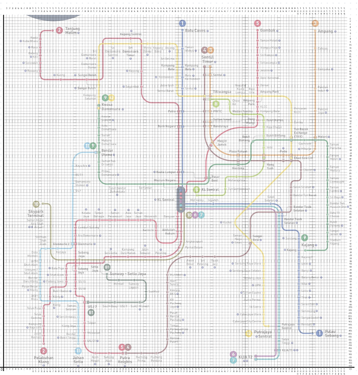
1. Copied the RapidKL MRT map and reduced its opacity.
2. Overlaid a grid on the map to determine approximate positions for each station.
3. Manually mapped each station as a node with its respective coordinates.

Graph Construction

Thus, each station in the MRT network is represented as a graph:

• Nodes: Represent MRT stations.
• Edges: Represent connections between stations.

Manually mapped nodes are structured as JSON objects, e.g.:

{
  "id": "titiwangsa",
  "connectedStations": ["batuCaves", "station2"],
  "data": {
    "label": "Titiwangsa",
    "lines": [
      { "color": "yellow", "stationNumber": 17 }
    ],
    "connectedStations": [
      { "id": "sentulBarat", "time": 2 },
      { "id": "hospitalKualaLumpur", "time": 2 }
    ]
  },
  "position": { "x": 6900, "y": 3000 }
}

Generating Edges

The ReactFlow library requires us to manually map out edges by defining an object that has a source node and target node. However, that process would have made this project much more harder to build with a lot of extra code. Thus, to make it more simpler I implemented the “connectedStations” and “lines” property in each station objects and used a function that would dynamically generate the stations edges.

This function would also generate the animated lines of stations that fall in the quickest path from two selected stations.

Pathfinding with A*

Illustration of A* search — https://en.wikipedia.org/wiki/A*_search_algorithm

The A* algorithm is the main feature of this whole program. It works similar to Djikstra’s algorithm but with a little add-on. In simple words, it finds the shortest path between two stations by evaluating two factors that combine together to form the formula:

𝑓(𝑛)=𝑔(𝑛)+ℎ(𝑛)

Where

• f(n) is the total estimated cost of the route across node
• g(n): The travel cost from the starting point to the current node.
• h(n): The heuristic estimate of the cost from the current node to the destination.

A heuristic in the A* algorithm is a guess about how close you are to the goal from a certain point. It helps the algorithm make smarter choices by guiding it toward the shortest path more efficiently.

Here I used the Euclidean distance (straight line draw from one node to the other) for the calculation of the heuristic. This value is derived from the x and y coordinates of each node.

Code for the heuristic calculation:

const calculateHeuristic = (currentNode, targetNode) => {
  const dx = currentNode.position.x - targetNode.position.x;
  const dy = currentNode.position.y - targetNode.position.y;
  return Math.sqrt(dx * dx + dy * dy);
};

Stations are explored using open and closed sets to avoid redundant evaluations, ensuring efficiency.

let currentNodeId = Array.from(openSet.entries()).reduce( (lowest, [id, node]) => 
!lowest || node.estimatedTotalCost < openSet.get(lowest)!.estimatedTotalCost ? 
id : lowest, null as string | null );

After the open set has been initialized it goes through a loop until there are no more options left in the open set. This is the key part of the algorithm. Where:

• The reduce() method goes through each entry in the openSet, comparing their estimatedTotalCost.
• The estimatedTotalCost is the sum of the cost it took to get to that node (cost) and an estimated distance to the target (using the heuristic function).
• The node with the lowest estimatedTotalCost is chosen as currentNodeId.

It continues until the current node is the same as the target. Once it is completed, it will push the node into the closed set.

Every time a node is visited and its neighbors are checked, the new nodes that appear in the search (which haven’t been visited or added to closedSet) are added to openSet.

At the end the path with the least cost is returned.

The Final UI

The final UI is a combination of the map with animated edges and a sidebar that displays the quickest math by mapping out the selected edges.

Final UI — Main Map Component, Top Bar for Input, and Sidebar for Simplified Path

Challenges Encountered

• Edge Duplication: Connections between stations often resulted in duplicate edges (e.g., A-B and B-A). This was resolved by comparing station IDs during edge creation.
• Interchange Stations: Overlapping edges in interchange stations required careful mapping to maintain clarity and correctness.
• Visual Path Clarity: Ensuring paths followed the MRT line colors without cluttering the map.

Takeaway

Through the use of open and closed sets, the algorithm avoids redundant exploration and ensures that the optimal path is found, even in large, complex networks. Whether applied in navigation, game development, or robotics, A* remains a cornerstone in pathfinding algorithms due to its balance of accuracy and performance.

This project showcases the power of combining graph theory and interactive tools to solve real-world problems. Using open and closed sets ensures efficient exploration, making the A* algorithm suitable for large, complex networks.

Future Enhancements:

• Create a data generator for JSON input, simplifying system design and reducing manual data entry.